[KT AIVLE] DX트랙 딥러닝(8주차) 복습(딥러닝 기초: Regression, 이진분류, 다중분류)

728x90

딥러닝 기초 복습

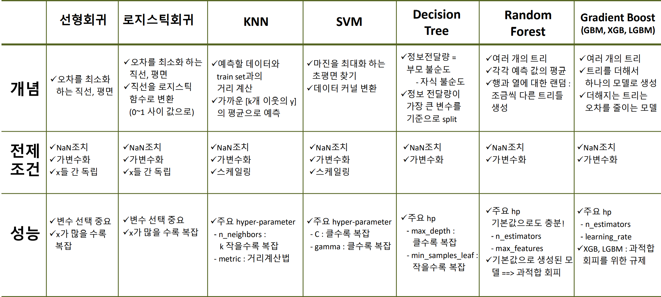
머신러닝 정리

알고리즘

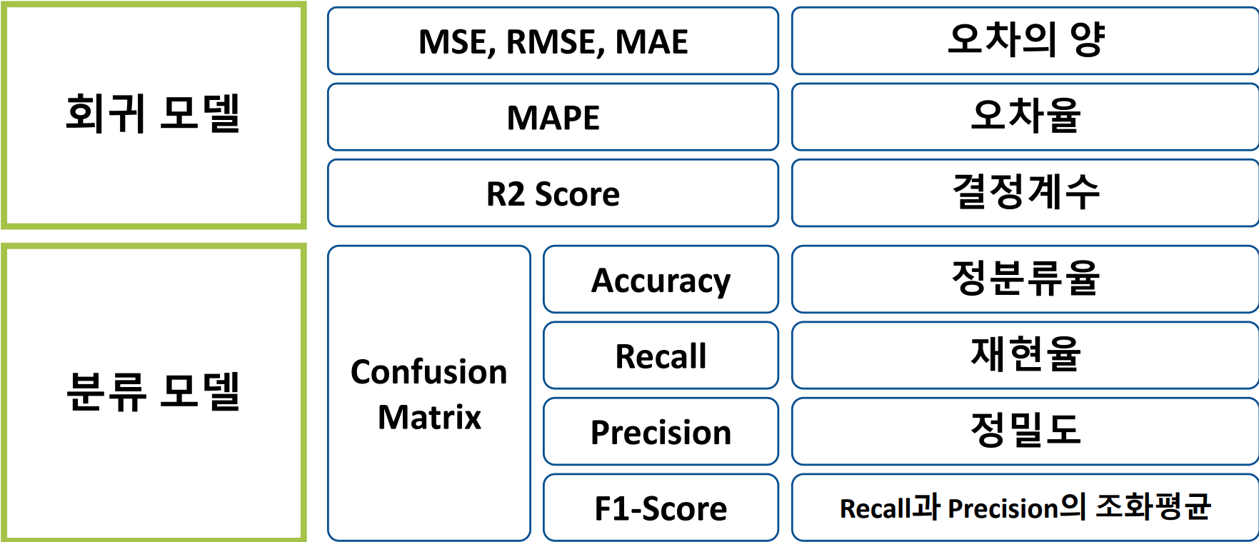
평가 지표

딥러닝 개념

인공 신경망을 사용하여 복잡한 패턴을 학습하고 데이터를 분석하는 기술
스케일링 필수

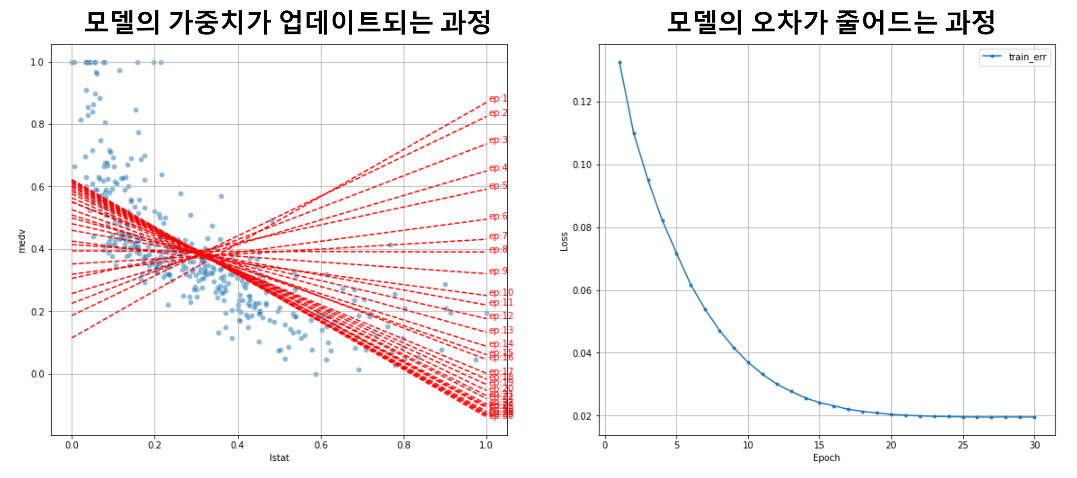
가중치 조정

조금씩 가중치(weight)를 조정하며 지정한 횟수나 더 이상 오차가 줄지 않을 때까지 오차 확인
- 이를 학습이라고 함(가장 적합한 가중치를 찾는 과정)

학습 절차

가중치에 초기값 할당
예측 결과 출력
오차 계산(MSE)
오차를 줄이는 방향으로 가중치(weight) 조정(가중치 = 파라미터)
1번으로 올라가 반복(max iteration에 도달)

loss function: 오차계산
optimizer: 가중치 조절
learning_rate: 학습율 결정
epoch: 반복횟수

딥러닝 모델링

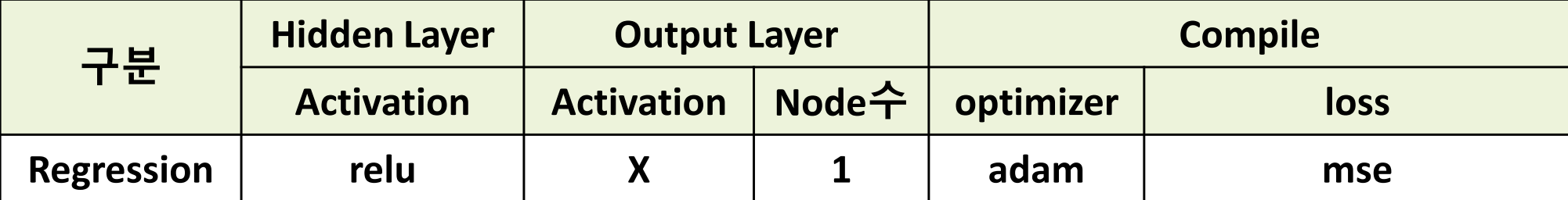
1. Regression

스케일링

# 스케일러 선언
scaler = MinMaxScaler()
# train 셋으로 fitting & 적용
x_train = scaler.fit_transform(x_train)
# validation 셋은 적용만
x_val = scaler.transform(x_val)

딥러닝 구조

이전 단계의 Output을 Input으로 받아 처리 후 전달
Input - Task1 - Task2 - ... - Output

딥러닝 코드 - Dense

# 메모리 정리
clear_session()

# Sequential 타입
model = Sequential([Dense(1, input_shape = (nfeatures,))]) # 1 = output, nfeatures = input

# 모델요약
model.summary()

input_shape =(,) : 분석단위 shape
- 1차원 : (feature 수, )
- 2차원 : (rows, columns)

딥러닝 코드 - Compile

model.compile(optimizer = Adam(learning_rate = 0.1) , loss='mse')

loss fuction(오차함수)
- 오차 계산을 무엇으로 할지 결정
- 회귀모델은 보통 mse 사용
optimizer
- 오차를 최소화 하도록 가중치를 조절하는 역할
- learning_rate 기본값 = 0.001

딥러닝 코드 - 학습, 학습곡선

history = model.fit(x_train, y_train, epochs = 20, validation_split = 0.2).history

epochs
- 가중치 조정 반복 횟수
- 전체 데이터를 몇 번 학습할 것인지 정해 줌
validation_split = 0.2
- train 데이터에서 20%를 검증셋으로 분리
.history
- 학습을 수행하면서 변화하는 가중치에 따른 성능 측정 및 기록

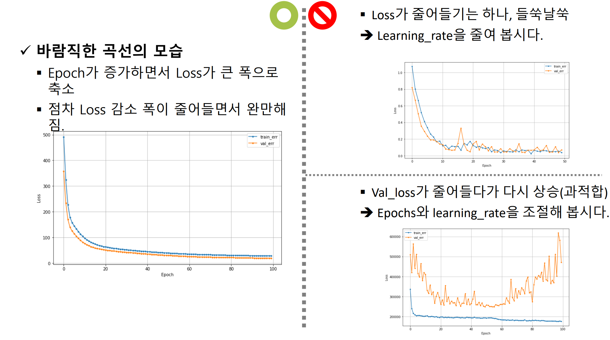
오차율(Loss)이 들쑥날쑥
- Learning_rate 조절
Val_loss가 줄어들다가 다시 상승(과적합)
- Epochs, learning_rate 조절

평가하기

R - squared(R²)

[평균 모델의 오차] 대비 [회귀모델이 해결한 오차 비율]
회귀모델이 얼마나 오차를 해결했는지를 나타냄
결정계수, 설명력

Hidden layer

model = Sequential([Dense(2, input_shape = (nfeatures,), activation = 'relu'
		, Dense(1)])

layer가 여러 개이면 리스트로 입력([])
Activation Function(활성 함수)
- hidden layer는 활성화 함수를 필요로 함(보통 relu)
- 선형함수를 비선형 함수로 변환해 주는 역할

1) 라이브러리 불러오기

import pandas as pd
import numpy as np
import matplotlib.pyplot as plt
import seaborn as sns

from sklearn.model_selection import train_test_split
from sklearn.metrics import *
from sklearn.preprocessing import MinMaxScaler

from keras.models import Sequential
from keras.layers import Dense
from keras.backend import clear_session
from keras.optimizers import Adam

2) 데이터 분할

target = '타겟 변수명' # y
features = ['lstat', 'ptratio', 'crim'] # x 
x = data.loc[:, features]
y = data.loc[:, target]

# 데이터 분할
x_train, x_val, y_train, y_val = train_test_split(x, y, test_size=.2, random_state = 20)

3) 스케일링

# 스케일러 선언
scaler = MinMaxScaler()

# train 셋으로 fitting & 적용
x_train = scaler.fit_transform(x_train)

# validation 셋은 적용만
x_val = scaler.transform(x_val)

4) 모델설계

# 분석단위의 shape
nfeatures = x_train.shape[1] #num of columns

# 메모리 정리
clear_session()

# Sequential 타입 
model = Sequential( Dense(1, input_shape = (nfeatures,)) )

# 모델요약
model.summary()

# 컴파일
model.compile(optimizer = Adam(learning_rate = 0.1), loss = 'mse')

5) 학습

# 학습
history = model.fit(x_train, y_train, 
                    epochs = 20, validation_split=0.2).history
                    
# 학습 결과 그래프
def dl_history_plot(history):
    plt.figure(figsize=(10,6))
    plt.plot(history['loss'], label='train_err', marker = '.')
    plt.plot(history['val_loss'], label='val_err', marker = '.')

    plt.ylabel('Loss')
    plt.xlabel('Epoch')
    plt.legend()
    plt.grid()
    plt.show()
    
dl_history_plot(history)

6) 예측

pred = model.predict(x_val)

print(f'RMSE : {mean_squared_error(y_val, pred, squared=False)}')
print(f'MAE  : {mean_absolute_error(y_val, pred)}')
print(f'MAPE : {mean_absolute_percentage_error(y_val, pred)}')

회귀 모델링 정리

2. 이진분류

Activation Function(활성 함수)

Hidden Layer

ReLU
- 좀 더 깊이 있는 학습을 시키기 위해 사용

Output Layer

이진분류 - Sigmoid
- 결과를 0, 1로 변환하기 위해 사용
다중분류 - softmax
- 각 범주에 대한 결과를 범주별 확률 값으로 변환

이진분류 모델에서의 compile

loss = binary_crossentropy
두 분포의 차이 계산

1) 라이브러리 로딩

import pandas as pd
import numpy as np
import matplotlib.pyplot as plt
import seaborn as sns

from sklearn.model_selection import train_test_split
from sklearn.metrics import *
from sklearn.preprocessing import MinMaxScaler

from keras.models import Sequential
from keras.layers import Dense
from keras.backend import clear_session
from keras.optimizers import Adam

2) 데이터 정리

target = 'Attrition'

# 불필요한 변수 제거
data.drop('EmployeeNumber', axis = 1, inplace = True)

x = data.drop(target, axis = 1)
y = data.loc[:, target]

3) 가변수화

범주형 데이터이면서 값이 0,1 로 되어 있는 것이 아니라면, 가변수화를 수행

dum_cols = ['BusinessTravel','Department','Education','EducationField','EnvironmentSatisfaction','Gender',
            'JobRole', 'JobInvolvement', 'JobSatisfaction', 'MaritalStatus', 'OverTime', 'RelationshipSatisfaction',
            'StockOptionLevel','WorkLifeBalance' ]

x = pd.get_dummies(x, columns = dum_cols ,drop_first = True)

4) 분할 및 스케일링

x_train, x_val, y_train, y_val = train_test_split(x, y, test_size = 200, random_state = 2022)

scaler = MinMaxScaler()
x_train = scaler.fit_transform(x_train)
x_val = scaler.transform(x_val)

5) 모델링

# input 확인
n = x_train.shape[1]

# 메모리 정리
clear_session()

# Sequential 모델 생성
model = Sequential([Dense( 16  , input_shape = (n, )   , activation = 'relu' ),
                    Dense( 8 ,  activation = 'relu' ),
                    Dense( 4 ,  activation = 'relu'),
                    Dense( 1 , activation= 'sigmoid')])

# 모델 요약
model.summary()

6) compile 및 학습

model.compile( optimizer = Adam(learning_rate = 0.001), loss = 'binary_crossentropy')
hist = model.fit( x_train, y_train, epochs = 50, validation_split= .2 ).history

7) 예측 및 검정

pred = model.predict(x_val)
pred = np.where( pred >= 0.5 , 1 , 0)

print(confusion_matrix(y_val, pred))
print(classification_report(y_val, pred))

이진분류 모델링 요약

3. 다중분류

Node 수

Output Layer의 node 수는 y의 범주 수와 같음

Softmax

Class 별(Output Node)로 예측한 값을, 하나의 확률 값으로 변환

다중 분류 전처리

정수인코딩(0부터시작) : sparse_categorical_crossentropy
One-hot Encoding : categorical_crossentropy

정수인코딩

sparse_categorical_crossentropy
y : Integer Encoding
- Target의 class들을 0부터 시작하여 순차 증가하는 정수로 인코딩
인코딩 된 범주 조회
- int_encoder.classes

from sklearn.preprocessing import LabelEncoder

# 선언
int_encoder = LabelEncoder()

# 인코딩
data['Species_encoded'] = int_encoder.fit_transform(data['Species'])
data.head()

원핫 인코딩

sklearn

from sklearn.preprocessing import OneHotEncoder

oh_encoder = OneHotEncoder()
#2차원
encoder_y1 = oh_encoder.fit_transform(data[['Species']])
print(encoded_y1.toarray())

2차원 구조로 입력해야 함

keras

from keras.utils import to_categorical

encoded_y2 = to_categorical(data['Species_encoded'],3)
print(encoded_y2)

정수 인코딩이 선행되어야 함

1) 데이터 준비

# np.argmax()
a = np.array([[1,2,3],[3,1,2]])
a

np.argmax(a, axis = 0) #열방향
np.argmax(a, axis = 1) #행방향
np.argmax(a) #2

2) sparse_categorical_crossentropy 사용을 위해 y값을 0, 1, 2로 변환

data['Species'] = data['Species'].map({'setosa':0, 'versicolor':1, 'virginica':2})

3) 데이터 분할

target = 'Species'
x = data.drop(target, axis = 1)
y = data.loc[:, target]

x_train, x_val, y_train, y_val = train_test_split(x, y, test_size = .3, random_state = 20)

4) 스케일링

scaler = MinMaxScaler()
x_train = scaler.fit_transform(x_train)
x_val = scaler.transform(x_val)